83. Robust Consumption Smoothing and Precautionary Savings#
83.1. Overview#
This lecture studies a robust version of the LQ permanent income model due to Hansen et al. [1999] and Hansen and Sargent [2008].
A consumer who distrusts his specification of the labor income process engages in a form of precautionary savings.
This is the third of four lectures on the LQ permanent income model.
It builds on The LQ Permanent Income Model, which develops the standard model, and Consumption Smoothing with Incomplete and Complete Markets, which studies its cross-section and market-structure implications.
The sequel, A Robust LQ Bewley Model, uses the results developed here to build a Bewley economy populated by consumers who differ in how much they distrust their income model.
Our description of the model with concerns about robustness includes
how, for quantities, a concern for robustness is observationally equivalent to an increase in impatience
how the worst-case model that the consumer uses to shape his decision rule distorts the baseline model’s endowment process toward greater persistence
a breakdown point beyond which the robust control problem ceases to have a solution
a frequency-domain representation of the effects of concerns about misspecification of the endowment process
a detection-error-probability characterization of the amount of model uncertainty
A recurring theme is that a single scalar \(\alpha^2\), the variance of the innovation to the consumer’s marginal utility, summarises everything about the endowment process that matters for robustness.
Let’s begin with some imports.
import numpy as np
import matplotlib.pyplot as plt
83.2. A brief review#
We recall the essentials from The LQ Permanent Income Model and Consumption Smoothing with Incomplete and Complete Markets.
83.2.1. Notation#
Because a robust decision maker guards against distortions to the mean of a shock, we need separate symbols for the shock and for the distortion.
We therefore adopt the following conventions, which differ in three places from the two preceding lectures.
Note
\(w_{t+1}\) is the baseline IID shock, as in The LQ Permanent Income Model, and \(v_{t+1}\) is a distortion to its conditional mean, as in Robust Permanent Income and Pricing.
\(\sigma \leq 0\) is the robustness parameter. The standard deviations of the two endowment shocks, written \(\sigma_1\) and \(\sigma_2\) in the preceding lectures, are renamed \(\eta_1\) and \(\eta_2\) here so that \(\sigma\) is free.
\(a_t\) denotes the consumer’s net assets, equal to minus the debt \(b_t\) of The LQ Permanent Income Model. This frees \(b_t\) for the preference shifter of Hansen et al. [1999].
83.2.2. The model#
A consumer with quadratic utility and discount factor \(\beta\) faces the endowment process
The optimal decision rule has a state-space representation in which the state is current consumption \(c_t\) and the exogenous endowment state \(z_t\):
We again use the two-factor endowment \(y_t = z_{1t} + z_{2t}\),
with \(z_{1t}\) a permanent component and \(z_{2t}\) a purely transitory component.
83.2.3. The consumption innovation#
One scalar built from (83.2) will do all of the work below.
The first line of (83.2) says that consumption is a random walk whose innovation is \(h\, w_{t+1}\), where
Define \(\alpha^2\) to be the variance of that innovation,
For the two-factor endowment (83.3) we have \(\check A = \mathrm{diag}(1,0)\), \(\check C = \mathrm{diag}(\eta_1,\eta_2)\) and \(\check G = \begin{pmatrix}1 & 1\end{pmatrix}\), so that \((I-\beta\check A)^{-1} = \mathrm{diag}\bigl((1-\beta)^{-1},1\bigr)\) and
The permanent shock variance \(\eta_1^2\) enters with coefficient \(1\) because a unit permanent shock is fully capitalised into consumption.
The transitory shock variance \(\eta_2^2\) enters with the small coefficient \((1-\beta)^2\) because only its annuity value is consumed.
This scalar does triple duty across the three lectures of this suite.
Note
\(\alpha^2\) is simultaneously
the variance of the consumption innovation in The LQ Permanent Income Model,
the rate at which the cross-section variance of consumption grows with age in Consumption Smoothing with Incomplete and Complete Markets, and
the quantity that, multiplied by \(\sigma\), governs every robustness result in this lecture.
Robust Permanent Income and Pricing writes the same object as \(\theta^2\).
The following cell fixes the calibration used below.
β = 0.95        # discount factor, so R = 1/β
η1 = 0.15       # std of permanent shock
η2 = 0.30       # std of transitory shock

R = 1 / β
α2 = η1**2 + (1 - β)**2 * η2**2
α = np.sqrt(α2)

print(f"α^2 = {α2:.6f}")
print(f"  permanent  η1^2         = {η1**2:.6f} "
      f"({100 * η1**2 / α2:5.1f}% of α^2)")
print(f"  transitory (1-β)^2 η2^2 = {(1 - β)**2 * η2**2:.6f} "
      f"({100 * (1 - β)**2 * η2**2 / α2:5.1f}% of α^2)")
α^2 = 0.022725
  permanent  η1^2         = 0.022500 ( 99.0% of α^2)
  transitory (1-β)^2 η2^2 = 0.000225 (  1.0% of α^2)
Permanent shocks account for almost all of \(\alpha^2\) in this calibration.
83.3. A robust permanent income model#
83.3.1. Robustness and precautionary savings#
We now study a consumer who distrusts his specification of the stochastic process governing his labor income.
The model is due to Hansen et al. [1999] (HST), who estimated it on US quarterly consumption and investment data.
For a fuller treatment of the HST model and its asset-pricing implications, see Robust Permanent Income and Pricing.
A consumer who fears model misspecification engages in a form of precautionary savings that is distinct from the usual precautionary motive, which requires a convex marginal utility.
Here, the precautionary motive arises because the consumer wants to protect against misspecification of the conditional means of income shocks, and it operates even with quadratic preferences.
HST showed an important observational equivalence result: for quantities \((c_t, i_t)\) alone, a concern for robustness is indistinguishable from an increase in impatience, that is, a decrease in \(\beta\).
We develop this result carefully below.
83.3.2. The HST model#
HST’s model features a planner with preferences over consumption streams \(\{c_t\}\), mediated through service streams \(\{s_t\}\).
Let \(b\) be a preference shifter, or utility bliss point.
The Bellman equation for the robust planner is
subject to the household technology, capital accumulation, endowment dynamics, and the state law:
Here \(^*\) denotes the next-period value; \(c\) is consumption; \(s\) is the scalar service measure; \(h\) is a habit stock; \(k\) is the capital stock; \(i\) is investment; \(d\) is an endowment shock; \(b\) is a preference shock; \(\gamma\) is the marginal product of capital; \(w^* \sim N(0,I)\) is the baseline shock; and \(v^*\) is a distortion to the conditional mean of \(w^*\) chosen by a minimizing agent.
The penalty parameter \(\theta\) governs the consumer’s concern about robustness.
A large \(\theta\) makes distortions expensive and so restrains the minimizing agent.
We use the transformation
so that \(\sigma = 0\), equivalently \(\theta = \infty\), corresponds to no robustness concern, and \(\sigma < 0\) to an increasing concern.
When \(\lambda > 0\) and \(\delta_h \in (0,1)\), the technology (83.8) accommodates habit persistence or durability, and the stock \(h_t\) is a geometric weighted average of current and past consumption.
Equation \(c_t + k_t = R k_{t-1} + d_t\) with \(R = \delta_k + \gamma\) combines capital accumulation with a linear production technology, so \(R\) is the physical gross return on capital.
Let \(x_t^\top = [h_{t-1},\, k_{t-1},\, z_t^\top]\).
The state transition equation is
where \(u_t = c_t\) and \(v_{t+1}\) is the distortion to the conditional mean of \(w_{t+1}\).
HST estimated the model on US quarterly data from 1970Q1 to 1996Q3, using nondurables plus services for consumption and durable consumption plus gross private investment for investment.
They imposed \(\beta R = 1\) and \(\delta_k = 0.975\), so \(\gamma\) is pinned down once \(\beta\) is estimated.
Two of their preference estimates are worth recording.
Parameter |
Habit |
No habit |
|---|---|---|
\(\beta\) |
0.997 |
0.997 |
\(\delta_h\) |
0.682 |
— |
\(\lambda\) |
2.443 |
0 |
\(2 \times \log L\) |
779.05 |
762.55 |
At a quarterly frequency, \(\beta = 0.997\) implies an annual real interest rate of \(\beta^{-4} - 1 \approx 1.2\%\).
The remaining estimated parameters govern the exogenous \(d_t\) and \(b_t\) processes and are reported in Appendix A of Hansen et al. [1999].
83.3.3. Solution when \(\sigma = 0\)#
When \(\sigma = 0\) the objective reduces to
Forming a Lagrangian and deriving first-order conditions yields
Here \(\mu_{st}\) is the marginal valuation of consumption services, which summarises the endogenous state variables \(h_{t-1}\) and \(k_{t-1}\).
The last line of (83.12) implies \(\mathbb{E}_t\mu_{c,t+1} = (\beta R)^{-1}\mu_{ct}\), so \(\mu_{st}\) is a martingale when \(\beta R = 1\):
for some vector \(\nu\).
Solving forward and substituting gives
where
and \(\tilde\delta_h = (\delta_h + \lambda)/(1+\lambda)\).
In the widely-studied special case \(\lambda = \delta_h = 0\), we have \(s_t = c_t\) and \(\mu_{st} = b_t - c_t\), and the marginal propensity to consume out of non-human wealth \(Rk_{t-1}\) equals that out of human wealth \(\sum_{j=0}^{\infty}R^{-j}\mathbb{E}_t d_{t+j}\), a well-known feature of the LQ model.
The formula for \(\mu_{st}\) can be written as \(\mu_{st} = M_s x_t\) where \(x_t\) follows (83.10).
It follows that
This \(\alpha\) is the same scalar we met in (83.5).
To see why, set \(\lambda = \delta_h = 0\) and hold \(b_t\) fixed, so that \(\mu_{st} = b - c_t\) and the innovation to \(\mu_{st}\) is minus the innovation to \(c_t\).
Hence \(\nu^\top = -h\) and \(\alpha^2 = \nu^\top\nu = h h^\top\), exactly as in (83.5).
The sign is irrelevant because only \(\alpha^2\) ever appears.
83.4. Observational equivalence#
HST state an observational-equivalence theorem.
Theorem 83.1 (Observational equivalence, I)
Fix all parameters except \((\sigma, \beta)\) and suppose \(\beta R = 1\) when \(\sigma = 0\).
There exists \(\underline\sigma < 0\) such that for any \(\sigma \in (\underline\sigma, 0)\), the optimal consumption-investment plan for \((0,\beta)\) is also chosen by a robust decision maker with parameters \((\sigma, \hat\beta(\sigma))\), where
and \(\hat\beta(\sigma) < \beta\).
The second equality in (83.17) uses \(R = \beta^{-1}\) and will be the form we use in computations.
Since \(R > 1\) and \(\alpha^2 > 0\), a more negative \(\sigma\), meaning a stronger robustness concern, lowers \(\hat\beta\).
A robust consumer wants to save more because his alter ego, a utility-minimizing agent, makes future income look worse than the approximating model predicts.
A lower discount factor makes a consumer less patient and therefore reduces saving.
When these two forces are balanced according to (83.17), consumption plans are identical across \((\sigma, \hat\beta(\sigma))\) pairs.
Proof. When \(\beta R = 1\) and \(\sigma = 0\), the marginal utility \(\mu_{st}\) obeys the martingale
where \(\tilde w_t\) is scalar IID with mean zero and unit variance.
Activating a concern about robustness, \(\sigma < 0\), leads the utility-minimizing alter ego to set
making the worst-case model for \(\mu_{st}\)
For the allocation to remain the same, we require the robust Euler equation \(\hat\beta R\,\hat{\mathbb{E}}_t\mu_{s,t+1} = \mu_{st}\) to hold under the worst-case model, which gives
The minimizing agent’s Bellman equation, a pure forecasting problem, yields
where \(P(\hat\beta)\) solves the scalar Bellman equation
Solving (83.21)-(83.23) for \(\hat\beta\) gives exactly (83.17).
Equation (83.17) is the useful numerical object because it gives a straight-line map from the robustness parameter to the observationally equivalent discount factor.
83.4.1. Precautionary savings interpretation#
The consumer’s concern about model misspecification activates the precautionary savings motive that underlies the observational-equivalence theorem.
A concern about robustness makes the consumer save more.
Decreasing \(\beta\) makes the consumer save less.
The observational-equivalence theorem says that these two forces can be made to offset each other exactly.
In the special case \(\lambda = \delta_h = 0\), \(s_t = c_t\) and the consumption rule is
The marginal propensity to consume out of non-human wealth \(Rk_{t-1}\) equals that out of human wealth \(\mathbb{E}_t\sum R^{-j}d_{t+j}\).
This equal-propensity property is a hallmark of the LQ model and persists when a concern for robustness is present, in contrast to usual precautionary-savings models with convex marginal utility.
Theorem 83.1 says that with \(\sigma < 0\), the observationally equivalent \(\hat\beta\) satisfies \(\hat\beta < \beta\).
If the starting point has \(\beta R = 1\), then \(\hat\beta R < 1\).
For a non-robust consumer with discount factor \(\hat\beta\) at the same interest rate, the Euler equation implies \(\mathbb{E}_t c_{t+1} < c_t\), so expected consumption declines over time.
This downward drift is the impatience offset in Theorem 83.1.
It cancels the robust consumer’s precautionary-savings motive, leaving the consumption and investment quantities unchanged.
The classical precautionary motive arises because
This channel requires convexity of marginal utility and is absent with quadratic preferences.
In contrast, the robustness-based precautionary motive operates through distortions of conditional means of shocks, shifting the first moment of the innovation to non-financial income.
83.4.2. Observational equivalence and distorted expectations#
The observational-equivalence result can be interpreted using a Stackelberg multiplier game.
After the minimizing agent has committed to a distortion process \(\{v_{t+1}\}\), the maximizing consumer faces the following worst-case law of motion for the state \(X_t\):
A robust consumer forms expectations of future income using the distorted transition matrix \(A - BF + CK\) rather than the approximating transition matrix \(A - BF\).
The distorted expectations operator \(\hat{\mathbb{E}}_t\) satisfies
Observational equivalence requires that the modified human-wealth formula
equals its benchmark counterpart \(\Psi_4 \sum_{j=0}^{\infty} R^{-j} \mathbb{E}_t d_{t+j}\).
This is achieved by a mutual adjustment of the coefficients \(\hat\Psi_j\) through \(\hat\beta\) and of the distorted expectation operator \(\hat{\mathbb{E}}_t\) through \(\sigma\).
The worst-case eigenvalue of \(A - BF + CK\) exceeds that of \(A - BF\) in modulus, so the worst-case distortions make the income process more persistent than under the approximating model.
This is the precautionary motive in state-space form: the minimizing agent makes future income look more risky by introducing low-frequency persistence.
In the scalar reduction of the next section, this eigenvalue is \(\zeta\), and we verify that \(\zeta > 1\) while the approximating model has a unit root.
83.4.3. Another observational equivalence result#
Theorem 83.2 (Observational equivalence, II)
Fix all parameters except \((\sigma,\beta)\) and consider a consumption-investment allocation for \((\hat\sigma, \hat\beta)\) where \(\hat\beta R = 1\) and \(\hat\sigma < 0\).
Then there exists \(\tilde\beta > \hat\beta\) such that the \((\hat\sigma, \hat\beta)\) allocation also solves the \((0, \tilde\beta)\) problem.
Theorem 83.1 showed that starting from a benchmark with \(\beta R = 1\), activating robustness is equivalent to reducing \(\beta\).
Theorem 83.2 goes in the opposite direction: the effects of activating a concern for robustness from a starting point with \(\beta R = 1\) are replicated by increasing \(\beta\) while setting \(\sigma = 0\).
In other words, when \(\beta R = 1\), a concern for robustness operates like an increase in the discount factor, pushing \(\beta R > 1\) and imparting an upward drift to the expected consumption profile.
Proof. With \(\hat\beta R = 1\) and \(\hat\sigma < 0\), the robust Euler equation implies
One seeks \(\tilde\beta > \hat\beta\) and \(\sigma = 0\) such that the same allocation solves the non-robust problem with discount factor \(\tilde\beta\).
The key step is to observe that the worst-case distortion \(K(\hat\sigma, \hat\beta)\) introduces a drift in the marginal utility process that is equivalent to the drift produced by raising the discount factor above \(\hat\beta\).
Equating the two drifts and solving the scalar Bellman equation for \(K\) yields
Setting \(\hat\sigma = 0\) makes the square root equal \((1-\hat\beta)/(1+\hat\beta)\), so that \(\tilde\beta = \hat\beta\).
Since \(1 + \hat\sigma\alpha^2\) decreases as \(\hat\sigma\) falls below zero, both the prefactor and the square root increase, so \(\tilde\beta > \hat\beta\) whenever \(\hat\sigma < 0\).
83.4.4. Comparing the two loci#
Both (83.17) and (83.30) are closed forms, so we can plot them directly.
We start from a benchmark with \(\beta R = 1\).
σ_grid = np.linspace(0.0, -0.16, 60)

# locus I: non-robust agent fixed at βR=1, report the robust twin's β̂(σ)
β_hat = β + σ_grid * α2 * β / (1 - β)

# locus II: robust agent fixed at βR=1, report the non-robust twin's β̃(σ̂)
q = 1 + σ_grid * α2
β_tilde = β * (1 + β) / (2 * q) * (1 + np.sqrt(1 - 4 * β * q / (1 + β)**2))

fig, ax = plt.subplots()
ax.plot(-σ_grid, β_hat, lw=2, color='C3',
        label=r'locus I: robust twin $\hat\beta(\sigma) < \beta$')
ax.plot(-σ_grid, β_tilde, lw=2, color='C0',
        label=r'locus II: non-robust twin $\tilde\beta(\hat\sigma) > \beta$')
ax.axhline(β, color='k', linestyle=':', lw=1,
           label=r'benchmark $\beta$ ($\beta R = 1$)')
ax.set_xlabel(r'robustness concern $|\sigma|$')
ax.set_ylabel('discount factor of the equivalent agent')
ax.legend()
plt.show()
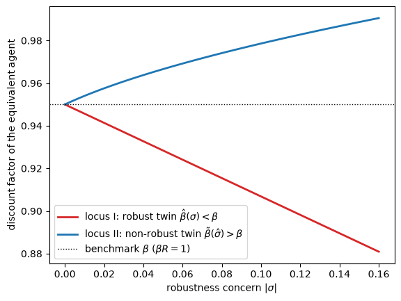
Fig. 83.1 Two observational-equivalence experiments. Locus I holds the non-robust agent fixed at \(\beta R = 1\) and reports the robust twin’s discount factor \(\hat\beta(\sigma)\); locus II holds the robust agent fixed at \(\beta R = 1\) and reports the non-robust twin’s discount factor \(\tilde\beta(\hat\sigma)\).#
Both loci pass through the benchmark \(\beta\) at \(\sigma = 0\) and separate as the robustness concern grows.
The key to reading Fig. 83.1 is that the two loci hold different agents fixed, so the discount factor plotted on the vertical axis refers to a different agent on each curve.
Locus I, from Theorem 83.1, holds the non-robust agent fixed at the benchmark \((\sigma = 0, \beta)\) with \(\beta R = 1\) and reports the discount factor \(\hat\beta(\sigma) < \beta\) of the robust agent that mimics it.
This is the sense in which HST call a concern for robustness observationally equivalent to a lower discount factor: because robustness already makes the agent save more, its discount factor must be lowered to hold the allocation at the benchmark.
Because the non-robust benchmark has \(\beta R = 1\), its optimal consumption is a martingale, \(\mathbb{E}_t c_{t+1} = c_t\).
The robust twin chooses the identical consumption process, so it too satisfies \(\mathbb{E}_t c_{t+1} = c_t\).
The lower \(\hat\beta\), which has \(\hat\beta R < 1\), would on its own impart a downward drift, but the robust agent’s precautionary saving offsets it exactly, leaving expected consumption flat.
Locus II, from Theorem 83.2, instead holds the robust agent fixed at \((\hat\sigma, \beta)\) with \(\beta R = 1\) and reports the discount factor \(\tilde\beta(\hat\sigma) > \beta\) of the non-robust agent that mimics it.
Here there is no impatience offset, so the common allocation inherits the robust agent’s precautionary upward drift, which the non-robust twin reproduces through \(\tilde\beta R > 1\).
The two experiments encode the same economics: a concern for robustness adds precautionary saving that acts like extra patience.
They differ only in which agent is anchored at \(\beta R = 1\), and hence in whether the common saving motive shows up as an exactly-offsetting impatience adjustment, as in locus I where expected consumption is flat, or as an upward drift in expected consumption, as in locus II.
83.5. The scalar worst-case model#
The proof of Theorem 83.1 reduced the robust problem to a scalar forecasting problem in the marginal utility \(\mu_{st}\).
That scalar problem can be solved in closed form, which is worth doing because it makes the worst-case dynamics, the breakdown point, and the frequency-domain results all transparent.
83.5.1. A closed-form solution#
Combining (83.21) with (83.17) and \(R = \beta^{-1}\) gives the worst-case persistence directly:
This is the central formula of the lecture.
The worst-case persistence of marginal utility is exactly the ratio of the two discount factors.
Since \(\hat\beta(\sigma) < \beta\) for \(\sigma<0\), we have \(\zeta(\sigma) > 1\): the approximating model for \(\mu_{st}\) has a unit root, and the worst-case model is mildly explosive.
That is the scalar counterpart of the statement in (83.26) that the worst-case transition matrix has a larger eigenvalue than the approximating one.
We can also solve (83.23) explicitly.
Write \(u = \sigma\alpha^2\) and \(\delta = 1-\beta\), so that (83.17) reads \(\hat\beta - 1 + u = (u - \delta^2)/\delta\).
The discriminant in (83.23) is then a perfect square:
so the two roots of (83.23) are available in closed form:
Substituting into (83.22), the first root reproduces (83.31) while the second gives the constant \(\zeta = R\), which violates the Euler equation (83.21) except at the single point where the two roots coincide.
So the economically relevant root is the constant \(P = -(1-\beta)^{-1}\), independent of \(\sigma\).
Note
Selecting the root numerically, by taking whichever of the two is closer to the target \((\hat\beta R)^{-1}\), is treacherous.
Because (83.32) is a perfect square, the square root is \(|u+\delta^2|/\delta\), and the sign in front of it that selects \(P = -(1-\beta)^{-1}\) flips as \(u\) crosses \(-\delta^2\).
A solver that picks the root by a distance criterion will silently switch branches there.
83.5.2. The breakdown point#
Theorem 83.1 asserts the existence of a lower bound \(\underline\sigma < 0\) without saying what it is.
The scalar model tells us.
The minimizing agent’s problem has a finite value only if the discounted worst-case state is square summable, that is, only if \(\hat\beta\,\zeta^2 < 1\).
Using \(\hat\beta = \beta/\zeta\) from (83.31), this condition is \(\beta\zeta < 1\), or equivalently \(\zeta < R\).
Substituting (83.31) and solving gives the breakdown point
At \(\sigma = \underline\sigma\) three things happen at once.
The discriminant (83.32) has a double root, so the two roots in (83.33) coincide.
The worst-case persistence reaches \(\zeta = R\), so \(\hat\beta\zeta^2 = 1\) exactly.
The observationally equivalent discount factor reaches \(\hat\beta = \beta^2\).
For \(\sigma < \underline\sigma\) the robust control problem has no solution, and any numerical answer reported there is meaningless.
We therefore restrict every plot below to \(\sigma \in (\underline\sigma, 0]\).
83.5.3. Verifying the closed form#
The following cell solves the quadratic (83.23) numerically and checks it against the closed forms (83.31) and (83.33).
def worst_case_persistence(σ, β, α2):
    """
    Worst-case persistence ζ(σ) of marginal utility on the
    observational-equivalence locus, from eq:rcs-zeta.
    """
    return 1 / (1 + σ * α2 / (1 - β))


def solve_scalar_riccati(σ, β, α2):
    """
    Solve the scalar Bellman equation eq:rcs-riccati by brute force and
    return both roots together with the implied persistence ζ = 1/(1-σα²P).
    """
    β_hat = β + σ * α2 * β / (1 - β)
    u = σ * α2
    disc = (β_hat - 1 + u)**2 + 4 * u
    roots = np.array([(β_hat - 1 + u + s * np.sqrt(disc)) / (-2 * u)
                      for s in (1.0, -1.0)])
    return roots, 1 / (1 - u * roots)


σ_lo = -(1 - β)**2 / α2               # breakdown point, eq:rcs-breakdown
print(f"breakdown point  σ̲  = {σ_lo:.6f}")
print(f"there            β̂  = {β + σ_lo * α2 * β / (1 - β):.6f} "
      f"(β² = {β**2:.6f})")
print(f"                 ζ   = {worst_case_persistence(σ_lo, β, α2):.6f} "
      f"(R = {R:.6f})")

print(f"\n{'σ':>10}{'P (numerical roots)':>28}{'-1/(1-β)':>12}"
      f"{'ζ (num)':>12}{'ζ (closed)':>12}")
for σ in [-0.02, -0.05, -0.09, -0.105]:
    roots, ζs = solve_scalar_riccati(σ, β, α2)
    keep = np.argmin(np.abs(roots + 1 / (1 - β)))
    print(f"{σ:10.3f}{str(np.round(roots, 4)):>28}{-1 / (1 - β):12.4f}"
          f"{ζs[keep]:12.6f}{worst_case_persistence(σ, β, α2):12.6f}")
breakdown point  σ̲  = -0.110011
there            β̂  = 0.902500 (β² = 0.902500)
                 ζ   = 1.052632 (R = 1.052632)

         σ         P (numerical roots)    -1/(1-β)     ζ (num)  ζ (closed)
    -0.020         [ -20.    -110.011]    -20.0000    1.009173    1.009173
    -0.050         [-20.     -44.0044]    -20.0000    1.023253    1.023253
    -0.090         [-20.     -24.4469]    -20.0000    1.042650    1.042650
    -0.105         [-20.     -20.9545]    -20.0000    1.050114    1.050114
One root is pinned at \(-(1-\beta)^{-1} = -20\) for every \(\sigma\), exactly as (83.33) predicts, and the implied \(\zeta\) agrees with the closed form to displayed precision.
Notice also that the two roots approach each other as \(\sigma\) falls toward \(\underline\sigma \approx -0.11\).
The next figure plots the worst-case impulse response \(\zeta^h\) over the admissible range.
horizons = np.arange(31)

fig, ax = plt.subplots()
for frac in [0.0, 0.4, 0.8, 0.98]:
    σ = frac * σ_lo
    ζ = worst_case_persistence(σ, β, α2)
    ax.plot(horizons, ζ**horizons, lw=2,
            label=rf'$\sigma={σ:.3f}$, $\zeta={ζ:.3f}$')

ax.set_xlabel('horizon $h$')
ax.set_ylabel(r'response of $\mu_{s,t+h}$')
ax.legend()
plt.show()
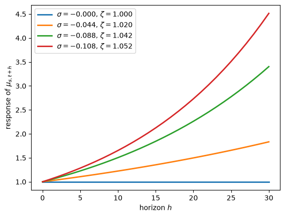
Fig. 83.2 Worst-case impulse response of marginal utility. The approximating model has a unit root; the worst-case model is increasingly explosive as \(\sigma\) falls toward the breakdown point \(\underline\sigma\).#
Fig. 83.2 shows that as \(\sigma\) falls, the minimizing agent converts the unit root of the approximating model into mild explosiveness.
At the breakdown point the response would grow at the gross interest rate \(R\), so that the discounted worst-case state ceases to be square summable.
83.6. Frequency domain interpretation#
The LQ permanent income framework has a natural frequency-domain interpretation.
The consumer’s concave utility makes him dislike high-frequency fluctuations in consumption, which he smooths by adjusting savings.
High-frequency fluctuations are easy to smooth, so the consumer is automatically robust to misspecification of high-frequency features of the income process.
Low-frequency fluctuations are harder to smooth because they are more persistent.
In the frequency-domain notation of HST, the transfer function from shocks \(w_t\) to the target \(s_t - b_t\) is \(G(\cdot)\), and the frequency decomposition of the \(H_2\) criterion is
The evaluation at \(\sqrt{\beta}\,e^{i\omega}\) rather than at \(e^{i\omega}\) is essential and not merely conventional.
Both the approximating model and the worst-case model for \(\mu_{st}\) are non-stationary, the first with a unit root and the second explosive, so neither has an ordinary spectral density.
Discounting by \(\sqrt\beta\) is exactly what makes the object in (83.35) finite.
In the scalar model of The scalar worst-case model, the target is \(s_t - b_t = -\mu_{st}\), and from (83.20) we can read off the transfer function and the discounted spectral density
This is finite precisely when \(\zeta\sqrt{\hat\beta} < 1\), which is the condition \(\hat\beta\zeta^2<1\) that defines the breakdown point (83.34).
So the frequency-domain object and the breakdown point are two views of the same restriction.
At \(\sigma = 0\) we have \(\zeta = 1\) and \(\hat\beta = \beta\), and (83.36) reduces to the discounted spectral density of a random walk.
ω = np.linspace(0, np.pi, 400)


def spectrum(σ, β, α2):
    ζ = worst_case_persistence(σ, β, α2)
    β_hat = β / ζ
    return α2 / np.abs(1 - ζ * np.sqrt(β_hat) * np.exp(1j * ω))**2


S0 = spectrum(0.0, β, α2)

fig, axes = plt.subplots(1, 2, figsize=(11, 4))

for frac in [0.0, 0.4, 0.8, 0.95]:
    σ = frac * σ_lo
    S = spectrum(σ, β, α2)
    axes[0].plot(ω, S, lw=2, label=rf'$\sigma={σ:.3f}$')
    axes[1].plot(ω, S / S0, lw=2, label=rf'$\sigma={σ:.3f}$')

axes[0].set_yscale('log')
axes[0].set_xlabel(r'frequency $\omega$')
axes[0].set_ylabel(r'$S(\omega;\sigma)$')
axes[0].set_title('discounted spectral density')
axes[0].legend()

axes[1].set_yscale('log')
axes[1].set_xlabel(r'frequency $\omega$')
axes[1].set_ylabel(r'$S(\omega;\sigma)\,/\,S(\omega;0)$')
axes[1].set_title('relative to the approximating model')
axes[1].legend()

fig.tight_layout()
plt.show()
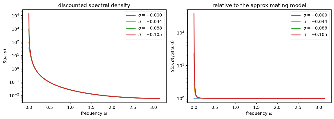
Fig. 83.3 Left: the discounted spectral density of the robust consumer’s target. Right: the same densities relative to the approximating model. The minimizing agent concentrates its distortion at low frequencies, where the permanent income consumer is least able to smooth.#
The left panel of Fig. 83.3 shows that \(S(\omega;\sigma)\) is largest at \(\omega \approx 0\), where the consumer’s welfare is most sensitive to income variability.
The right panel makes the key point: the ratio \(S(\omega;\sigma)/S(\omega;0)\) is sharply decreasing in \(\omega\).
Recognizing where the consumer is vulnerable, the minimizing agent concentrates the worst-case distortions at low frequencies, and it does so more aggressively as \(|\sigma|\) grows.
The peak at \(\omega = 0\) equals \(\alpha^2/(1-\sqrt{\beta\zeta})^2\) and diverges as \(\sigma \to \underline\sigma\), which is another way of seeing the breakdown point.
Because the distortion is \(v_t = K\mu_{s,t-1}\) by (83.19), the spectral density of the distortion process is \(K^2\) times the density of \(\mu_{s,t-1}\), so it inherits the same low-frequency concentration.
83.7. Detection error probabilities#
A natural way to discipline the choice of \(\sigma\) is to ask: how difficult would it be to distinguish the approximating model from the worst-case model statistically?
For a sample of length \(T\), one can use a log-likelihood ratio test to compare the two hypotheses.
The detection error probability (DEP) is the probability of making the wrong decision using the log-likelihood ratio statistic when one does not know which model generated the data:
When \(\sigma = 0\) the two models are identical and \(\mathrm{DEP} = 0.5\).
As \(|\sigma|\) increases the models diverge and the DEP falls toward zero.
In the scalar model the two hypotheses are fully explicit:
Both have Gaussian innovations with the same variance \(\alpha^2\), so the log-likelihood ratio is a difference of sums of squares.
def simulate_paths(ζ, α, T, n_paths, seed):
    "Simulate n_paths draws of μ_{t+1} = ζ μ_t + α w_{t+1} from μ_0 = 0."
    rng = np.random.default_rng(seed)
    paths = np.zeros((n_paths, T + 1))
    shocks = rng.standard_normal((n_paths, T))
    for t in range(T):
        paths[:, t + 1] = ζ * paths[:, t] + α * shocks[:, t]
    return paths


def log_likelihood_ratio(paths, ζ, α):
    "Return log p_worst(path) - log p_approx(path)."
    lag, lead = paths[:, :-1], paths[:, 1:]
    return 0.5 * (np.sum(((lead - lag) / α)**2, axis=1)
                  - np.sum(((lead - ζ * lag) / α)**2, axis=1))


def detection_error_probability(ζ, α, T=40, n_paths=10_000, seed=1234):
    "Finite-sample DEP for the approximating and worst-case scalar laws."
    if np.isclose(ζ, 1.0):
        return 0.5
    approx = simulate_paths(1.0, α, T, n_paths, seed)
    worst = simulate_paths(ζ, α, T, n_paths, seed + 1)
    return 0.5 * (np.mean(log_likelihood_ratio(worst, ζ, α) < 0)
                  + np.mean(log_likelihood_ratio(approx, ζ, α) > 0))
We use \(T = 40\), which is ten years of quarterly data.
Before plotting, it is worth noting a property that makes the DEP the right way to report a robustness concern.
The parameter \(\sigma\) is not scale free: it always enters through the product \(\sigma\alpha^2\), and \(\alpha^2\) has the units of consumption squared.
Doubling the units in which consumption is measured therefore changes the numerical value of \(\sigma\) that represents a given concern for robustness.
The DEP has no such problem, because \(\alpha\) cancels from the likelihood ratio in (83.38).
ζ_test = worst_case_persistence(0.6 * σ_lo, β, α2)
for scale in [0.5, 1.0, 2.0]:
    dep = detection_error_probability(ζ_test, scale * α)
    print(f"α scaled by {scale:>4}:  DEP = {dep:.4f}")
α scaled by  0.5:  DEP = 0.3334
α scaled by  1.0:  DEP = 0.3334
α scaled by  2.0:  DEP = 0.3334
The DEP depends only on \(\zeta\) and on the sample size \(T\).
σ_vals = np.linspace(0.0, 0.999 * σ_lo, 31)
ζ_vals = worst_case_persistence(σ_vals, β, α2)

fig, ax = plt.subplots()
for T, color in [(40, 'C0'), (160, 'C2')]:
    dep_vals = np.array([detection_error_probability(ζ, α, T=T)
                         for ζ in ζ_vals])
    ax.plot(-σ_vals, dep_vals, lw=2, color=color, label=f'$T = {T}$')

ax.axhline(0.2, color='C3', linestyle='--', lw=1.2, label='DEP = 0.2')
ax.axvline(-σ_lo, color='k', linestyle=':', lw=1,
           label='breakdown point')
ax.set_xlabel(r'robustness concern $|\sigma|$')
ax.set_ylabel('detection error probability')
ax.set_ylim(0.0, 0.52)
ax.legend()
plt.show()
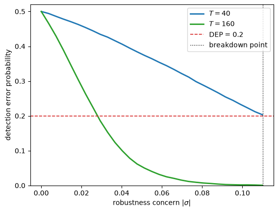
Fig. 83.4 Finite-sample detection error probability against the robustness concern, over the admissible range \((\underline\sigma, 0]\), for two sample lengths. Values below the dashed line are the ones HST regard as implausible, because the approximating and worst-case models would then be too easy to tell apart.#
Note
HST suggested that a DEP above 0.2 is “plausible”, meaning the models are still hard enough to distinguish statistically that a concern for robustness is warranted.
Values of \(\sigma\) with \(\mathrm{DEP} \geq 0.2\) therefore define a set of plausible worst-case models.
Fig. 83.4 shows that the two disciplines interact in an interesting way.
At \(T = 40\) the DEP curve reaches the \(0.2\) threshold essentially exactly at the breakdown point.
In other words, with ten years of quarterly data, every robustness concern that this model can represent at all is also statistically plausible: the mathematical limit binds first, and the statistical one is slack.
for frac in [0.6, 0.9, 0.999]:
    ζ = worst_case_persistence(frac * σ_lo, β, α2)
    print(f"σ = {frac * σ_lo:.5f} (= {frac:.3f} σ̲):  "
          f"DEP = {detection_error_probability(ζ, α):.4f}")
σ = -0.06601 (= 0.600 σ̲):  DEP = 0.3334
σ = -0.09901 (= 0.900 σ̲):  DEP = 0.2329
σ = -0.10990 (= 0.999 σ̲):  DEP = 0.2034
That near-coincidence is a property of this calibration and of \(T = 40\), not a theorem.
At \(T = 160\) the ordering reverses, and statistical detectability binds well before the breakdown point.
σ_report = 0.6 * σ_lo
ζ_report = worst_case_persistence(σ_report, β, α2)
print(f"at σ = {σ_report:.4f}  (ζ = {ζ_report:.4f}):")
for T in [20, 40, 80, 160]:
    print(f"  T = {T:>3}:  DEP = "
          f"{detection_error_probability(ζ_report, α, T=T):.4f}")
at σ = -0.0660  (ζ = 1.0309):
  T =  20:  DEP = 0.4147
  T =  40:  DEP = 0.3334
  T =  80:  DEP = 0.1507
  T = 160:  DEP = 0.0203
The lesson is that the plausible amount of model uncertainty depends on how much data the econometrician is imagined to have.
83.8. Robustness of decision rules#
A natural follow-up question is whether robust decision rules perform better than the non-robust rule when the data are in fact generated by a distorted model.
Define the payoff when the decision rule is designed for robustness parameter \(\sigma^r\) and the data are generated by the distorted model associated with \(\sigma^d\):
where the state evolves under decision rule \(F(\sigma^r)\) and worst-case shocks \(K(\sigma^d)\):
There is an important caveat about which family of rules to compare, and it follows directly from Theorem 83.1.
Along the observational-equivalence locus \((\sigma, \hat\beta(\sigma))\), every agent chooses the same decision rule.
So \(F(\sigma^r)\) does not vary along the locus, and \(\pi(\sigma^d;\sigma^r)\) is constant in \(\sigma^r\) there.
A meaningful comparison of rules must therefore move off the locus, for example by holding \(\beta\) fixed at the benchmark and varying \(\sigma^r\) alone.
That experiment requires solving the full HST matrix problem rather than the scalar reduction of The scalar worst-case model, because once we leave the locus the marginal-utility process no longer summarises the decision rule.
Robust Permanent Income and Pricing carries out that computation with the QuantEcon LQ and robust-control routines.
83.9. Concluding remarks#
A concern for model misspecification, parameterised by \(\sigma = -\theta^{-1} \leq 0\), alters the permanent income model in ways that are subtle rather than dramatic.
A concern for robustness generates a precautionary savings motive even under quadratic preferences, by distorting the conditional means of income shocks.
The distorted worst-case model makes the income process more persistent, shifting power toward the low frequencies where the permanent income consumer is most vulnerable.
The observational equivalence theorem Theorem 83.1 shows that for quantities \((c_t, i_t)\) alone, a concern for robustness is indistinguishable from a reduction in \(\beta\).
The reverse theorem Theorem 83.2 shows that, starting from \(\beta R = 1\), robustness is observationally equivalent to an increase in \(\beta\), which imparts an upward drift to expected consumption.
Two disciplines bound how large a robustness concern can sensibly be.
The breakdown point (83.34) is a hard mathematical limit beyond which no solution exists.
Detection error probabilities provide a softer and scale-free statistical discipline: choose \(|\sigma|\) small enough that the approximating and worst-case models remain difficult to distinguish.
The observationally equivalent \((\sigma, \hat\beta)\) pairs do have different implications for asset prices, a point pursued in Robust Permanent Income and Pricing.
They also have different implications for the beliefs that agents hold, which is the subject of A Robust LQ Bewley Model.
83.10. Exercises#
Exercise 83.1
This exercise derives the breakdown point (83.34).
Using (83.31), show that \(\hat\beta(\sigma)\,\zeta(\sigma)^2 = \beta\,\zeta(\sigma)\).
The minimizing agent’s problem has a finite value only if \(\hat\beta\zeta^2 < 1\). Use part 1 to show that this is equivalent to \(\zeta < R\), and hence that \(\underline\sigma = -(1-\beta)^2/\alpha^2\).
Verify that \(\hat\beta(\underline\sigma) = \beta^2\).
Explain why the breakdown point moves toward zero when the endowment becomes more volatile.
Solution
Here is one solution.
From (83.31), \(\zeta = \beta/\hat\beta\), so \(\hat\beta = \beta/\zeta\) and therefore \(\hat\beta\zeta^2 = (\beta/\zeta)\zeta^2 = \beta\zeta\).
By part 1 the condition \(\hat\beta\zeta^2 < 1\) is \(\beta\zeta < 1\), that is, \(\zeta < \beta^{-1} = R\).
Substituting the closed form (83.31) gives
\[ \left[1 + \frac{\sigma\alpha^2}{1-\beta}\right]^{-1} < \frac{1}{\beta} \iff 1 + \frac{\sigma\alpha^2}{1-\beta} > \beta \iff \sigma\alpha^2 > -(1-\beta)^2 , \]which is \(\sigma > -(1-\beta)^2/\alpha^2 = \underline\sigma\).
At \(\sigma = \underline\sigma\) we have \(\sigma\alpha^2 = -(1-\beta)^2\), so \(\zeta = [1-(1-\beta)]^{-1} = \beta^{-1} = R\) and \(\hat\beta = \beta/\zeta = \beta^2\).
A more volatile endowment raises \(\alpha^2\), and \(\underline\sigma = -(1-\beta)^2/\alpha^2\) is therefore closer to zero.
The economics is that \(\sigma\) only ever matters through \(\sigma\alpha^2\), so when the consumer faces more income risk a smaller \(|\sigma|\) already buys a given amount of pessimism.
Exercise 83.2
This exercise explains why a naive numerical solver for (83.23) misbehaves.
Verify algebraically that on the locus (83.17) the discriminant of (83.23) equals \(\bigl[(\sigma\alpha^2+(1-\beta)^2)/(1-\beta)\bigr]^2\).
Conclude that the square root equals \(|\sigma\alpha^2+(1-\beta)^2|/(1-\beta)\) and hence that the two roots are those in (83.33).
Write code that, for a grid of \(\sigma\) in \((\underline\sigma,0)\), records which sign in front of the square root in (83.23) yields the economically relevant root \(P=-(1-\beta)^{-1}\).
Confirm that the answer flips at \(\sigma = \underline\sigma\).
Solution
Here is one solution.
With \(u = \sigma\alpha^2\) and \(\delta = 1-\beta\), equation (83.17) gives \(\hat\beta - 1 = -\delta + u/\delta \cdot \beta/\beta\), more directly \(\hat\beta-1+u = (u-\delta^2)/\delta\).
Hence the discriminant is
\[ \frac{(u-\delta^2)^2}{\delta^2} + 4u = \frac{(u-\delta^2)^2 + 4u\delta^2}{\delta^2} = \frac{(u+\delta^2)^2}{\delta^2} . \]Taking the square root gives \(|u+\delta^2|/\delta\), and substituting the two signs into (83.23) gives \(P = -1/\delta\) and \(P = \delta/u\).
The sign flips exactly where \(u + \delta^2\) changes sign, that is at \(u = -\delta^2\), which is \(\sigma = \underline\sigma\).
σ_test = np.linspace(-0.01, 1.4 * σ_lo, 40)
signs = []
for σ in σ_test:
    roots, _ = solve_scalar_riccati(σ, β, α2)
    signs.append('+' if np.argmin(np.abs(roots + 1 / (1 - β))) == 0 else '-')

print(''.join(signs))
flip = next(i for i in range(1, len(signs)) if signs[i] != signs[i - 1])
print(f"sign flips between σ = {σ_test[flip - 1]:.5f} "
      f"and σ = {σ_test[flip]:.5f}")
print(f"breakdown point σ̲ = {σ_lo:.5f}")
++++++++++++++++++++++++++++------------
sign flips between σ = -0.10970 and σ = -0.11340
breakdown point σ̲ = -0.11001
Exercise 83.3
This exercise calibrates \(\sigma\) using the detection error probability.
Write a bisection that finds the \(\sigma\) at which \(\mathrm{DEP}(\sigma) = 0.2\), and report the associated \(\hat\beta\), \(\zeta\), and the ratio \(\sigma/\underline\sigma\).
Run it for \(T = 40\) and \(T = 160\).
Take care: the target need not be attained on the admissible range \((\underline\sigma, 0]\), and your code should say so rather than silently return an endpoint.
Solution
The DEP is decreasing in \(|\sigma|\), so a bisection works, but we must first check that the target lies within reach.
def σ_for_target_dep(target, T, β, α2, tol=1e-5):
    """
    Find σ ∈ (σ̲, 0) with DEP(σ) = target by bisection.

    Returns None if the DEP never falls to the target on the admissible
    range, which happens when the breakdown point binds before statistical
    detectability does.
    """
    α_loc = np.sqrt(α2)
    lo, hi = 0.999 * (-(1 - β)**2 / α2), 0.0     # lo is the more negative end

    def dep_at(σ):
        return detection_error_probability(
            worst_case_persistence(σ, β, α2), α_loc, T=T)

    if dep_at(lo) > target:
        return None

    while hi - lo > tol:
        mid = 0.5 * (lo + hi)
        if dep_at(mid) < target:
            lo = mid                # too easy to detect, move toward zero
        else:
            hi = mid
    return 0.5 * (lo + hi)


for T in [40, 160]:
    σ_star = σ_for_target_dep(0.2, T, β, α2)
    if σ_star is None:
        print(f"T = {T:>3}:  DEP stays above 0.2 on the whole admissible "
              f"range; the breakdown point binds first")
    else:
        ζ_star = worst_case_persistence(σ_star, β, α2)
        print(f"T = {T:>3}:  σ = {σ_star:.5f}   β̂ = {β / ζ_star:.5f}   "
              f"ζ = {ζ_star:.5f}   σ/σ̲ = {σ_star / σ_lo:.3f}")
T =  40:  DEP stays above 0.2 on the whole admissible range; the breakdown point binds first
T = 160:  σ = -0.02806   β̂ = 0.93788   ζ = 1.01292   σ/σ̲ = 0.255
A longer sample makes the two models easier to distinguish, so the \(\sigma\) that keeps the DEP at \(0.2\) moves closer to zero.
At \(T = 40\) no admissible \(\sigma\) has a DEP as low as \(0.2\), so the breakdown point is the binding constraint.
At \(T = 160\) statistical detectability binds first, at about a quarter of the way to the breakdown point.