48. Vector Autoregressions for Subsets of Variables#
In addition to what’s in Anaconda, this lecture will need the following libraries:
!pip install quantecon
48.1. Overview#
An economic model delivers a vector autoregression for a list of variables \(Y_t\).
An econometrician often observes only some of them.
This lecture answers three questions about that situation.
Given an \(m\)th order VAR for an \(n \times 1\) vector \(Y_t\) and a selector matrix \(S_y\) that extracts an \(n_y \times 1\) subvector \(y_t = S_y Y_t\):
What vector autoregression does \(y_t\) obey?
What is its moving average representation?
How are the innovations in the small system related to the innovations in the large one?
The answers all come from the Kalman filter.
The state is the history of \(Y_t\) that a finite-order VAR requires, and the observation is the subvector \(y_t\).
Because \(y_t\) is a subvector of the state and not a noisy signal about it, this is a state space system with no measurement error.
The main results are
\(y_t\) obeys an infinite-order VAR whose coefficients we compute exactly,
the innovation \(a_t\) of the small system is a one-sided distributed lag of the innovations \(\varepsilon_t\) of the large system,
that distributed lag has a wide coefficient matrix at every lag, so \(\varepsilon_t\) cannot be recovered from the history of \(y_t\),
the forecast error variance of the small system exceeds that of the large one by a quantity we compute.
Two special cases where the small VAR stays finite-order are identified and verified.
This lecture generalizes the worked example that used to close The Kalman Filter and Vector Autoregressions.
Let’s start with imports.
import matplotlib.pyplot as plt
import numpy as np
import quantecon as qe

plt.rcParams['figure.figsize'] = (10, 5)
np.set_printoptions(precision=4, suppress=True)
48.2. The large system#
Let \(Y_t\) be \(n \times 1\) and suppose it obeys the \(m\)th order vector autoregression
where \(\{\varepsilon_t\}\) is a serially uncorrelated sequence with \(\mathbb{E}[\varepsilon_{t+1} \mid Y_t, Y_{t-1}, \ldots] = 0\).
Stack \(m\) lags into the \(nm \times 1\) state vector
Then (48.1) becomes the first-order companion form
We write \(A\) without a subscript for the companion matrix and \(A_1, \ldots, A_m\) with subscripts for the VAR coefficient matrices.
Let \(J = \begin{pmatrix} I_n & 0 & \cdots & 0\end{pmatrix}\) be the \(n \times nm\) matrix that reads \(Y_t\) off the state, so that \(Y_t = J X_t\) and \(C = J^\top\).
We assume all eigenvalues of \(A\) are strictly inside the unit circle, so \(\{Y_t\}\) is covariance stationary.
48.3. The small system#
The econometrician observes
where \(S_y\) is \(n_y \times n\) with \(n_y < n\).
Usually \(S_y\) picks out \(n_y\) coordinates of \(Y_t\), but nothing below requires that, so linear combinations are allowed too.
Equations (48.2) and (48.3) are a state space system of the form studied in The Kalman Filter and Vector Autoregressions, with shock loading \(C\), observation matrix \(G\), and measurement error covariance
The observation is exact, but it is a strict subvector of the state, so the econometrician still faces a filtering problem.
Let \(\Sigma\) solve the steady-state Riccati equation
with associated Kalman gain
Here \(\Sigma\) is the covariance matrix of \(X_t - \mathbb{E}[X_t \mid y^{t-1}]\).
Note
Because \(X_t\) contains lags of \(Y_t\) whose \(S_y\) components the econometrician has already seen exactly, \(\Sigma\) is singular.
That is harmless.
What the Kalman gain (48.5) requires is that the innovation covariance \(G \Sigma G^\top\) be nonsingular, which holds whenever no linear combination of \(y_t\) is perfectly predictable from \(y^{t-1}\).
The innovation in the small system is
48.4. Four representations#
48.4.1. The Wold representation#
The steady-state innovations representation derived in The Kalman Filter and Vector Autoregressions is
Solving (48.7) forward gives the moving average representation of \(y_t\) in terms of its own innovations,
48.4.2. The vector autoregression#
Solving (48.7) backward instead gives
This is an infinite-order VAR, convergent because the eigenvalues of \(A - KG\) lie inside the unit circle.
48.4.3. Innovations of the small system in terms of the large one#
This is the question that motivates the lecture.
Let \(e_t = X_t - \hat X_t\) be the filtering error.
Subtracting the Kalman recursion \(\hat X_{t+1} = A \hat X_t + K a_t\) from the state equation (48.2) and using \(a_t = G e_t\) gives
Solving (48.10) backward and premultiplying by \(G\) yields the answer.
Proposition 48.1
The innovations of the small system are the one-sided distributed lag
of the innovations of the large system, with leading coefficient
Since each \(\Gamma_j\) is \(n_y \times n\) with \(n_y < n\), the map from \(\{\varepsilon_t\}\) to \(\{a_t\}\) has no inverse.
Knowing the entire history of \(y_t\) is not enough to recover \(\varepsilon_t\).
48.4.4. The structural moving average#
For comparison, iterating (48.2) gives \(y_t\) directly in terms of the large system’s innovations,
48.4.5. A forecast error that contains past shocks#
Separating the \(j = 0\) term in (48.11) and using \(\Gamma_0 = S_y\) gives
The first term is what it appears to be.
Because \(\mathbb{E}[\varepsilon_t \mid Y^{t-1}] = 0\), we have \(y_t - \mathbb{E}[y_t \mid Y^{t-1}] = S_y \varepsilon_t\), so \(S_y \varepsilon_t\) is the error made in forecasting \(y_t\) by someone who observes the entire history of \(Y\).
The second term deserves a pause, because at first sight it looks impossible.
By construction \(a_t\) is a forecast error, orthogonal to everything known at \(t-1\).
Yet (48.13) says that \(a_t\) loads on \(\varepsilon_{t-1}, \varepsilon_{t-2}, \ldots\), shocks that had already been realized by then.
The two facts are consistent, and both are true:
The resolution is that past shocks are known to the large system’s econometrician, not to the small one.
The small econometrician’s information set is \(H(y^{t-1})\), the closed linear span of \(y_{t-1}, y_{t-2}, \ldots\), and \(\varepsilon_{t-j}\) does not lie in it.
Let \(P_{t-1}\) denote projection onto \(H(y^{t-1})\).
Applying \(P_{t-1}\) to (48.13), using \(P_{t-1} a_t = 0\) and \(P_{t-1}\varepsilon_t = 0\), delivers the identity
So the distributed lag in (48.13) loads only on the parts of past shocks that the small econometrician has not yet learned,
A shock that happened three quarters ago can still be news today, if the only series you watch has not finished revealing it.
That is the whole content of the filtering problem, and it is why \(\Omega\) exceeds \(S_y V S_y^\top\).
48.4.6. What the coefficients \(\Gamma_j\) are#
Substituting the moving average (48.12) into the autoregression (48.9) and matching the coefficient on \(\varepsilon_{t-k}\) gives a second formula for the same objects,
So \(\Gamma_k\) measures the failure of the small system’s own autoregression to reproduce the large system’s \(k\)-lag response.
The case \(k = 1\) is worth writing out.
Since \(\Phi_0 = S_y\) and \(\Phi_1 = G A C = S_y A_1\),
Suppose \(S_y\) selects coordinates, and partition \(Y_t = (y_t^\top, \tilde y_t^\top)^\top\) as before.
Then \(B_1 S_y\) has zeros in the columns belonging to the dropped variables, so (48.18) reads
The loading of \(a_t\) on last period’s omitted shocks is exactly \(A_1^{y\tilde y}\), the block through which the omitted variables enter the retained equations.
Equation (48.19) also previews Proposition 48.3: block exogeneity sets \(A_1^{y\tilde y} = 0\), which forces \(B_1 = A_1^{yy}\) and hence \(\Gamma_1 = 0\).
48.4.7. A factorization identity#
Representations (48.8), (48.11), and (48.12) describe the same process, so with \(\Psi(z) = \sum_h \Psi_h z^h\) and similarly for \(\Gamma\) and \(\Phi\),
Equation (48.20) says the structural moving average operator factors into the Wold operator of the small system times the innovation map.
It is a sharp numerical check on everything above, and we use it as one.
Matching variances at each lag also gives
Every term in the second sum is positive semidefinite, so
The small system’s one-step forecast error variance is never smaller than the corresponding block of the large system’s, and (48.21) says exactly how much is lost.
48.5. Two cases where nothing is lost#
Proposition 48.2
If \(S_y = I_n\), then \(\Gamma_0 = I_n\) and \(\Gamma_j = 0\) for \(j \geq 1\), so \(a_t = \varepsilon_t\), and (48.9) collapses to the original \(m\)th order VAR (48.1).
Nothing is hidden, so the Wold innovations are the structural innovations.
The second case is more interesting.
Partition \(Y_t = (y_t^\top, \tilde y_t^\top)^\top\) and correspondingly
Proposition 48.3
Suppose \(y_t\) is block exogenous, meaning \(A_k^{y\tilde y} = 0\) for all \(k\), so that no lag of the omitted variables appears in the equations for \(y\).
Then \(\Gamma_j = 0\) for \(j \geq 1\), \(a_t = S_y \varepsilon_t\), \(\Omega = S_y V S_y^\top\), and \(y_t\) obeys the finite \(m\)th order VAR
Proof. Block exogeneity makes the \(y\) rows of (48.1) read \(y_{t+1} = \sum_k A_k^{yy} y_{t+1-k} + S_y \varepsilon_{t+1}\).
The right side involves only lags of \(y\), and \(S_y \varepsilon_{t+1}\) is orthogonal to the whole history \(Y^t\) and hence to \(y^t\).
So this is the projection of \(y_{t+1}\) on \(y^t\), which identifies it as the Wold representation.
Note what Proposition 48.3 does not require: \(V\) need not be block diagonal.
Contemporaneous correlation between \(\varepsilon^y\) and \(\varepsilon^{\tilde y}\) is fine.
What matters for whether an omitted variable damages a VAR is Granger causality, not contemporaneous correlation.
48.6. Code#
The class below packages everything.
class VARSubsystem:
    """
    A VAR for Y and the implied representations for a subvector y = S_y Y.

        Y[t+1] = A_1 Y[t] + ... + A_m Y[t-m+1] + eps[t+1],  E eps eps' = V
        y[t]   = S_y Y[t]

    Parameters
    ----------
    A_list : list of (n, n) arrays, the VAR coefficient matrices A_1, ..., A_m
    V      : (n, n) array, covariance matrix of eps
    S_y    : (n_y, n) selector matrix
    """

    def __init__(self, A_list, V, S_y):
        self.A_list = [np.atleast_2d(np.asarray(a, dtype=float)) for a in A_list]
        self.V = np.atleast_2d(np.asarray(V, dtype=float))
        self.S_y = np.atleast_2d(np.asarray(S_y, dtype=float))
        n, m = self.A_list[0].shape[0], len(self.A_list)
        self.n, self.m, self.n_y = n, m, self.S_y.shape[0]

        # companion form
        self.A = np.zeros((n * m, n * m))
        self.A[:n] = np.hstack(self.A_list)
        if m > 1:
            self.A[n:, :n * (m - 1)] = np.eye(n * (m - 1))
        self.J = np.zeros((n, n * m))
        self.J[:, :n] = np.eye(n)
        self.C = self.J.T
        self.G = self.S_y @ self.J
        self.Q = self.C @ self.V @ self.C.T
        self._Sigma = self._K = None

    def companion_eigenvalues(self):
        return np.linalg.eigvals(self.A)

    def stationary_filter(self):
        """Steady-state (Sigma, K) from the Riccati equation with R = 0."""
        if self._Sigma is None:
            A, G = self.A, self.G
            R = np.zeros((self.n_y, self.n_y))
            Sigma = qe.solve_discrete_riccati(A.T, G.T, self.Q, R)
            Omega = G @ Sigma @ G.T
            self._Sigma = Sigma
            self._K = A @ Sigma @ G.T @ np.linalg.inv(Omega)
        return self._Sigma, self._K

    def innovation_cov(self):
        """Omega = E a a', the one-step forecast error covariance of y."""
        Sigma, _ = self.stationary_filter()
        return self.G @ Sigma @ self.G.T

    def wold(self, h_max=20):
        """Psi[h] in y[t] = sum_h Psi[h] a[t-h]; Psi[0] = I."""
        _, K = self.stationary_filter()
        Psi = np.empty((h_max + 1, self.n_y, self.n_y))
        Psi[0], P = np.eye(self.n_y), np.eye(self.A.shape[0])
        for h in range(1, h_max + 1):
            Psi[h] = self.G @ P @ K
            P = P @ self.A
        return Psi

    def var_coefficients(self, h_max=20):
        """B[j-1] in y[t] = sum_j B[j] y[t-j] + a[t], for j = 1, ..., h_max."""
        _, K = self.stationary_filter()
        M = self.A - K @ self.G
        B, P = np.empty((h_max, self.n_y, self.n_y)), np.eye(self.A.shape[0])
        for j in range(h_max):
            B[j] = self.G @ P @ K
            P = P @ M
        return B

    def innovation_map(self, h_max=20):
        """Gamma[j] in a[t] = sum_j Gamma[j] eps[t-j]."""
        _, K = self.stationary_filter()
        M = self.A - K @ self.G
        Gamma, P = np.empty((h_max + 1, self.n_y, self.n)), np.eye(self.A.shape[0])
        for j in range(h_max + 1):
            Gamma[j] = self.G @ P @ self.C
            P = P @ M
        return Gamma

    def structural_ma(self, h_max=20):
        """Phi[j] in y[t] = sum_j Phi[j] eps[t-j]."""
        Phi, P = np.empty((h_max + 1, self.n_y, self.n)), np.eye(self.A.shape[0])
        for j in range(h_max + 1):
            Phi[j] = self.G @ P @ self.C
            P = P @ self.A
        return Phi

    def simulate(self, T, seed=0, burn=200):
        """Simulate Y and the innovations eps that generated it."""
        rng = np.random.default_rng(seed)
        L = np.linalg.cholesky(self.V)
        eps = rng.standard_normal((T + burn, self.n)) @ L.T
        X, Y = np.zeros(self.n * self.m), np.zeros((T + burn, self.n))
        for t in range(T + burn):
            X = self.A @ X + self.C @ eps[t]
            Y[t] = self.J @ X
        return Y[burn:], eps[burn:]

    def filter_innovations(self, y_path):
        """Recover a[t] from observed y by running the steady-state filter."""
        _, K = self.stationary_filter()
        x_hat = np.zeros(self.A.shape[0])
        a = np.empty((len(y_path), self.n_y))
        for t in range(len(y_path)):
            a[t] = y_path[t] - self.G @ x_hat
            x_hat = self.A @ x_hat + K @ a[t]
        return a


def convolve(Psi, Gamma, h_max):
    """(Psi * Gamma)[h] = sum_{k=0}^{h} Psi[k] Gamma[h-k]."""
    out = np.zeros((h_max + 1, Psi.shape[1], Gamma.shape[2]))
    for h in range(h_max + 1):
        for k in range(h + 1):
            out[h] += Psi[k] @ Gamma[h - k]
    return out
A single routine collects the diagnostics we want to see for every example.
def report(model, h_max=30, label=''):
    """Print the identities that every subsystem must satisfy."""
    Sigma, K = model.stationary_filter()
    A, G, V = model.A, model.G, model.V
    resid = Sigma - (A @ Sigma @ A.T + model.Q
                     - A @ Sigma @ G.T @ np.linalg.inv(G @ Sigma @ G.T)
                       @ G @ Sigma @ A.T)
    Psi = model.wold(h_max)
    Gamma = model.innovation_map(h_max)
    Phi = model.structural_ma(h_max)
    Omega, Vy = model.innovation_cov(), model.S_y @ V @ model.S_y.T

    print(f'--- {label} (n = {model.n}, m = {model.m}, n_y = {model.n_y})')
    print(f'  max |eig| of companion A      {np.max(abs(model.companion_eigenvalues())):.6f}')
    print(f'  max |eig| of A - KG           {np.max(abs(np.linalg.eigvals(A - K @ G))):.6f}')
    print(f'  Riccati residual              {np.abs(resid).max():.2e}')
    print(f'  |Gamma[0] - S_y|              {np.abs(Gamma[0] - model.S_y).max():.2e}')
    print(f'  |Phi - Psi * Gamma|           '
          f'{np.abs(convolve(Psi, Gamma, h_max) - Phi).max():.2e}')
    Gamma_long = model.innovation_map(300)      # the sum in (SS) is infinite
    print(f'  |Omega - sum Gamma V Gamma\'|  '
          f'{np.abs(Omega - sum(Gamma_long[j] @ V @ Gamma_long[j].T for j in range(301))).max():.2e}')
    print(f'  max |Gamma[j]|, j >= 1        {np.abs(Gamma[1:]).max():.3e}')
    print(f'  det Omega / det S_y V S_y\'    '
          f'{np.linalg.det(Omega) / np.linalg.det(Vy):.4f}')
    return Psi, Gamma, Phi
48.7. Example 1: a bivariate VAR(2)#
Two observable series \(r_t\) and \(z_t\) obey the VAR(2)
with
Note that \(z\) is block exogenous: its equation contains no lags of \(r\).
But \(r\) is not, since \(z\) enters the \(r\) equation with both lags.
So dropping \(z\) should matter, while dropping \(r\) should not.
A1 = np.array([[0.80,  0.75],
               [0.00,  0.75]])
A2 = np.array([[0.05, -0.72],
               [0.00,  0.20]])
V2 = np.eye(2)

S_both = np.eye(2)                    # observe (r, z)
S_r    = np.array([[1.0, 0.0]])       # observe r only
S_z    = np.array([[0.0, 1.0]])       # observe z only

mod_both = VARSubsystem([A1, A2], V2, S_both)
mod_r    = VARSubsystem([A1, A2], V2, S_r)
mod_z    = VARSubsystem([A1, A2], V2, S_z)

Psi_both, Gam_both, _ = report(mod_both, label='observe r and z')
print()
Psi_r, Gam_r, _ = report(mod_r, label='observe r only')
print()
Psi_z, Gam_z, _ = report(mod_z, label='observe z only')
--- observe r and z (n = 2, m = 2, n_y = 2)
  max |eig| of companion A      0.958631
  max |eig| of A - KG           0.000000
  Riccati residual              0.00e+00
  |Gamma[0] - S_y|              0.00e+00
  |Phi - Psi * Gamma|           0.00e+00
  |Omega - sum Gamma V Gamma'|  0.00e+00
  max |Gamma[j]|, j >= 1        0.000e+00
  det Omega / det S_y V S_y'    1.0000

--- observe r only (n = 2, m = 2, n_y = 1)
  max |eig| of companion A      0.958631
  max |eig| of A - KG           0.959007
  Riccati residual              1.78e-15
  |Gamma[0] - S_y|              0.00e+00
  |Phi - Psi * Gamma|           2.22e-16
  |Omega - sum Gamma V Gamma'|  2.00e-15
  max |Gamma[j]|, j >= 1        7.500e-01
  det Omega / det S_y V S_y'    1.5786

--- observe z only (n = 2, m = 2, n_y = 1)
  max |eig| of companion A      0.958631
  max |eig| of A - KG           0.858258
  Riccati residual              4.44e-16
  |Gamma[0] - S_y|              0.00e+00
  |Phi - Psi * Gamma|           0.00e+00
  |Omega - sum Gamma V Gamma'|  0.00e+00
  max |Gamma[j]|, j >= 1        0.000e+00
  det Omega / det S_y V S_y'    1.0000
Every identity holds to machine precision.
The three cases differ exactly as the propositions predict.
Observing both variables gives \(\Gamma_j = 0\) for \(j \geq 1\), so \(a_t = \varepsilon_t\), as Proposition 48.2 requires.
Observing only \(z\), which is block exogenous, also gives \(\Gamma_j = 0\) for \(j \geq 1\), so \(a_t = \varepsilon_{z,t}\), as Proposition 48.3 requires.
Observing only \(r\) is different.
Here \(\Gamma_j \neq 0\) for \(j \geq 1\), and the ratio of forecast error variances reports how much the \(r\)-only econometrician loses.
print('observe r only:')
print(f'  Omega           = {mod_r.innovation_cov()[0, 0]:.4f}')
print(f'  S_y V S_y\'      = {(S_r @ V2 @ S_r.T)[0, 0]:.4f}')
print('\n  Gamma[j] for j = 0, ..., 5 (rows: response of a to eps_r, eps_z)')
print(Gam_r[:6, 0, :])
observe r only:
  Omega           = 1.5786
  S_y V S_y'      = 1.0000

  Gamma[j] for j = 0, ..., 5 (rows: response of a to eps_r, eps_z)
[[ 1.      0.    ]
 [ 0.0769  0.75  ]
 [-0.0097 -0.0998]
 [ 0.0017  0.0125]
 [ 0.0002 -0.0023]
 [ 0.0004 -0.0003]]
The forecast error variance is over 50 percent larger than \(V_{11}\).
The extra variance is entirely attributable to past \(\varepsilon_z\) shocks that the econometrician sees only through their effect on \(r\).
48.7.1. The VAR for the subsystem#
B_r = mod_r.var_coefficients(12)

fig, ax = plt.subplots()
ax.stem(np.arange(1, 13), B_r[:, 0, 0], basefmt=' ')
ax.axhline(0, color='k', lw=0.6)
ax.set_xlabel('lag $j$')
ax.set_ylabel('$B_j$')
ax.set_title(r'Population VAR coefficients for $r_t$ when only $r$ is observed')
fig.tight_layout()
plt.show()

print('B_1, ..., B_6:', np.round(B_r[:6, 0, 0], 5))
print('\nfor comparison, A_1[0,0] and A_2[0,0]:', A1[0, 0], A2[0, 0])
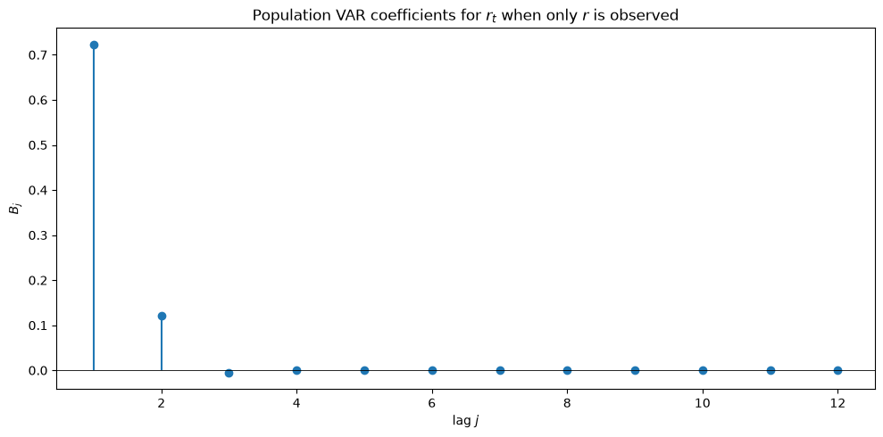
Fig. 48.1 VAR coefficients for the subsystem#
B_1, ..., B_6: [ 0.7231  0.1212 -0.0056  0.0007 -0.0001 -0.    ]

for comparison, A_1[0,0] and A_2[0,0]: 0.8 0.05
The infinite-order VAR for \(r\) alone is dominated by two lags, but neither coefficient equals the corresponding coefficient in the bivariate system.
Dropping \(z\) does not simply delete the \(z\) columns of the VAR; it changes what is left.
48.7.2. Wold impulse responses#
H = 25
h = np.arange(H + 1)
Psi_both = mod_both.wold(H)

fig, axes = plt.subplots(2, 2, figsize=(10, 6), sharex=True)
names, shocks = [r'$r_t$', r'$z_t$'], [r'$a_{r,t}$', r'$a_{z,t}$']
for i in range(2):
    for j in range(2):
        axes[i, j].plot(h, Psi_both[:, i, j], lw=2)
        axes[i, j].axhline(0, color='k', lw=0.6, ls='--')
        axes[i, j].set_title(f'{names[i]} to {shocks[j]}', fontsize=10)
        if i == 1:
            axes[i, j].set_xlabel('horizon $h$')
fig.suptitle('Wold responses, both variables observed')
fig.tight_layout()
plt.show()
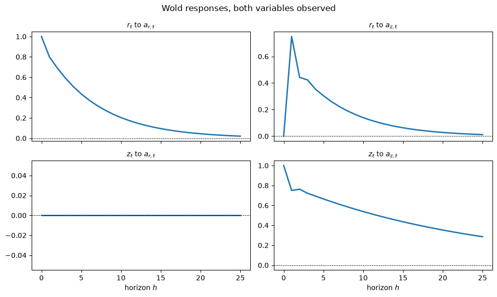
Fig. 48.2 Wold responses when both variables are observed#
Because \(a_t = \varepsilon_t\) here, these Wold responses coincide with the structural responses of the bivariate VAR.
Psi_r = mod_r.wold(H)
Phi_r = mod_r.structural_ma(H)

fig, ax = plt.subplots()
ax.plot(h, Psi_r[:, 0, 0], lw=2, label=r'$\Psi_h$: $r_t$ to its own innovation $a_t$')
ax.plot(h, Phi_r[:, 0, 0], lw=2, ls='--',
        label=r'$\Phi_h$: $r_t$ to $\varepsilon_{r,t}$')
ax.plot(h, Phi_r[:, 0, 1], lw=2, ls=':',
        label=r'$\Phi_h$: $r_t$ to $\varepsilon_{z,t}$')
ax.axhline(0, color='k', lw=0.6)
ax.set_xlabel('horizon $h$')
ax.set_ylabel('response')
ax.set_title(r'Wold versus structural responses of $r_t$')
ax.legend()
fig.tight_layout()
plt.show()
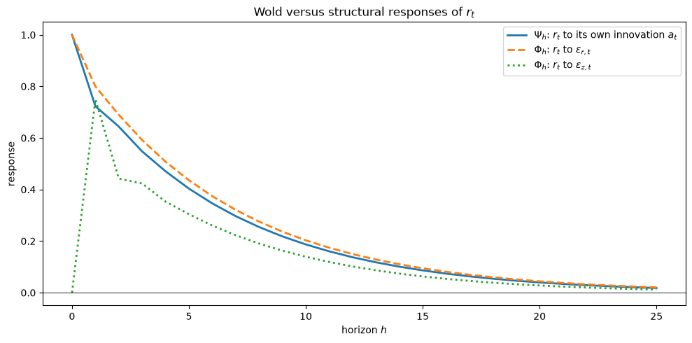
Fig. 48.3 Wold response when only r is observed#
The Wold response to \(a_t\) is not the response to either structural shock.
It is a blend, and (48.20) says exactly how the blending works.
48.7.3. Checking the innovation map by simulation#
Proposition Proposition 48.1 is a statement about population objects.
We check it on a long simulated sample by comparing the innovations that the Kalman filter extracts from the observed \(r\) series with the distributed lag \(\sum_j \Gamma_j \varepsilon_{t-j}\) built from the shocks that generated it.
T = 100_000
Y_sim, eps_sim = mod_r.simulate(T, seed=1)
y_sim = Y_sim @ S_r.T

a_filtered = mod_r.filter_innovations(y_sim)

J_lag = 400          # the distributed lag is infinite, so truncate generously
Gam_long = mod_r.innovation_map(J_lag)
a_theory = np.zeros_like(a_filtered)
for j in range(J_lag + 1):
    a_theory[j:] += eps_sim[:T - j] @ Gam_long[j].T

burn = J_lag + 1
print(f'correlation of the two series   '
      f'{np.corrcoef(a_filtered[burn:, 0], a_theory[burn:, 0])[0, 1]:.8f}')
print(f'max absolute difference         '
      f'{np.abs(a_filtered[burn:] - a_theory[burn:]).max():.2e}')
print(f'sample variance of a            {a_filtered[burn:, 0].var():.4f}')
print(f'population Omega                {mod_r.innovation_cov()[0, 0]:.4f}')
print(f'sample corr(a_t, a_(t-1))       '
      f'{np.corrcoef(a_filtered[burn + 1:, 0], a_filtered[burn:-1, 0])[0, 1]:.4f}')
correlation of the two series   1.00000000
max absolute difference         6.45e-10
sample variance of a            1.5706
population Omega                1.5786
sample corr(a_t, a_(t-1))       -0.0048
The two constructions of \(a_t\) agree to the accuracy of the truncated distributed lag, the sample variance of \(a_t\) matches \(\Omega\), and \(a_t\) is serially uncorrelated.
48.7.4. The two orthogonality facts#
Now we check (48.14) directly, by running two regressions on the simulated data.
The first regresses \(a_t\) on current and lagged structural shocks, which the small econometrician cannot see.
The second regresses \(a_t\) on lagged observations, which are all that the small econometrician can see.
P_lags = 4
Z_eps = np.column_stack([eps_sim[P_lags - l:T - l] for l in range(P_lags + 1)])
target = a_filtered[P_lags:, 0]
b_eps = np.linalg.lstsq(Z_eps, target, rcond=None)[0].reshape(P_lags + 1, 2)
fit = Z_eps @ b_eps.ravel()
r2_eps = 1 - ((target - fit) ** 2).sum() / target.var() / len(target)

print('OLS of a_t on eps_t, ..., eps_{t-4}:')
print(b_eps)
print('population Gamma_0, ..., Gamma_4:')
print(Gam_long[:P_lags + 1, 0, :])
print(f'max discrepancy {np.abs(b_eps - Gam_long[:P_lags + 1, 0, :]).max():.2e}')
print(f'R^2 = {r2_eps:.6f}')
OLS of a_t on eps_t, ..., eps_{t-4}:
[[ 1.     -0.    ]
 [ 0.0769  0.75  ]
 [-0.0097 -0.0998]
 [ 0.0017  0.0125]
 [ 0.0002 -0.0023]]
population Gamma_0, ..., Gamma_4:
[[ 1.      0.    ]
 [ 0.0769  0.75  ]
 [-0.0097 -0.0998]
 [ 0.0017  0.0125]
 [ 0.0002 -0.0023]]
max discrepancy 1.64e-05
R^2 = 0.999996
Q_lags = 8
Z_y = np.column_stack([y_sim[Q_lags - l - 1:T - l - 1, 0] for l in range(Q_lags)])
tgt = a_filtered[Q_lags:, 0]
b_y = np.linalg.lstsq(Z_y, tgt, rcond=None)[0]
resid = tgt - Z_y @ b_y
r2_y = 1 - (resid ** 2).sum() / tgt.var() / len(tgt)

print('OLS of a_t on y_{t-1}, ..., y_{t-8}:')
print(np.round(b_y, 5))
print(f'R^2 = {r2_y:.6f}')
OLS of a_t on y_{t-1}, ..., y_{t-8}:
[-0.0046  0.0044 -0.0015  0.001   0.0018 -0.0063  0.0055 -0.0024]
R^2 = 0.000056
The first regression recovers the \(\Gamma_j\) and fits almost perfectly, the small shortfall coming only from truncating the distributed lag at four lags.
So \(a_t\) really is built out of shocks stretching back before \(t\).
The second explains essentially nothing, confirming that \(a_t\) is nonetheless orthogonal to the small econometrician’s information set.
We can see why by asking how much of each past shock the small econometrician has managed to learn.
print('R^2 from projecting a structural shock on y_{t-1}, ..., y_{t-8}')
for lag in [0, 1, 2, 3]:
    r2s = []
    for k in range(2):
        shock = eps_sim[Q_lags - lag:T - lag, k]
        c = np.linalg.lstsq(Z_y, shock, rcond=None)[0]
        e = shock - Z_y @ c
        r2s.append(1 - (e ** 2).sum() / shock.var() / len(shock))
    print(f'   eps_(t-{lag}):   eps_r {r2s[0]:6.4f}    eps_z {r2s[1]:6.4f}')
R^2 from projecting a structural shock on y_{t-1}, ..., y_{t-8}
   eps_(t-0):   eps_r 0.0000    eps_z 0.0001
   eps_(t-1):   eps_r 0.6314    eps_z 0.0001
   eps_(t-2):   eps_r 0.6351    eps_z 0.3561
   eps_(t-3):   eps_r 0.6352    eps_z 0.3624
The current shock \(\varepsilon_t\) is entirely unpredictable from \(y^{t-1}\), as it must be.
Shocks from two or more periods back are substantially learned.
The interesting row is \(\varepsilon_{t-1}\): its \(r\) component is largely known, while its \(z\) component is completely unknown, because \(z_{t-1}\) reaches \(r\) only with a one-period lag and so has not yet shown up anywhere in \(y^{t-1}\).
That is why (48.19) gives \(a_t\) a loading on \(\varepsilon_{z,t-1}\) equal to the full structural coefficient \(A_1^{y\tilde y} = 0.75\), while its loading on \(\varepsilon_{r,t-1}\) is only the much smaller residual \(A_1^{yy} - B_1\).
B1 = mod_r.var_coefficients(1)[0]
print(f'Gamma_1                  = {Gam_long[1, 0, :]}')
print(f'[A1[0,0] - B_1,  A1[0,1]] = '
      f'[{A1[0, 0] - B1[0, 0]:.4f}, {A1[0, 1]:.4f}]')

Phi_r = mod_r.structural_ma(6)
B_r6 = mod_r.var_coefficients(6)
recursion = np.array([Phi_r[k] - sum(B_r6[j - 1] @ Phi_r[k - j]
                                     for j in range(1, k + 1))
                      for k in range(7)])
print(f'\nmax |Gamma_k - (Phi_k - sum_j B_j Phi_(k-j))| = '
      f'{np.abs(recursion - Gam_long[:7]).max():.2e}')
Gamma_1                  = [0.0769 0.75  ]
[A1[0,0] - B_1,  A1[0,1]] = [0.0769, 0.7500]

max |Gamma_k - (Phi_k - sum_j B_j Phi_(k-j))| = 1.25e-16
48.8. Example 2: an omitted interest rate#
Now a trivariate VAR(1) in output growth \(g_t\), inflation \(\pi_t\), and an interest rate \(i_t\), from which the econometrician drops \(i_t\).
We contrast two coefficient matrices that differ only in whether the interest rate feeds back onto \(g\) and \(\pi\).
The shock covariance matrix \(V\) is the same in both, and it is not diagonal, so the interest rate innovation is contemporaneously correlated with the other two.
V3 = np.array([[0.36, 0.05, 0.02],
               [0.05, 0.25, 0.06],
               [0.02, 0.06, 0.16]])
S_gpi = np.array([[1.0, 0.0, 0.0],
                  [0.0, 1.0, 0.0]])

A_exog = np.array([[0.60, 0.10, 0.00],
                   [0.15, 0.55, 0.00],
                   [0.30, 0.40, 0.70]])
A_fb = np.array([[0.60, 0.10, -0.35],
                 [0.15, 0.55,  0.25],
                 [0.30, 0.40,  0.70]])

mod_exog = VARSubsystem([A_exog], V3, S_gpi)
mod_fb = VARSubsystem([A_fb], V3, S_gpi)

_, Gam_exog, _ = report(mod_exog, label='i is block exogenous')
print()
_, Gam_fb, _ = report(mod_fb, label='i feeds back')
--- i is block exogenous (n = 3, m = 1, n_y = 2)
  max |eig| of companion A      0.700000
  max |eig| of A - KG           0.700000
  Riccati residual              5.55e-17
  |Gamma[0] - S_y|              0.00e+00
  |Phi - Psi * Gamma|           2.78e-17
  |Omega - sum Gamma V Gamma'|  0.00e+00
  max |Gamma[j]|, j >= 1        1.110e-16
  det Omega / det S_y V S_y'    1.0000

--- i feeds back (n = 3, m = 1, n_y = 2)
  max |eig| of companion A      0.792688
  max |eig| of A - KG           0.558938
  Riccati residual              1.11e-16
  |Gamma[0] - S_y|              0.00e+00
  |Phi - Psi * Gamma|           1.11e-16
  |Omega - sum Gamma V Gamma'|  1.11e-16
  max |Gamma[j]|, j >= 1        3.500e-01
  det Omega / det S_y V S_y'    1.1614
The block exogenous case behaves exactly as Proposition 48.3 says it must, despite the correlated shocks.
The feedback case does not.
print('block exogenous: B_1 versus the (g, pi) block of A_1')
print(mod_exog.var_coefficients(3)[0])
print(A_exog[:2, :2])
print(f'  max |B_j| for j >= 2: {np.abs(mod_exog.var_coefficients(12)[1:]).max():.2e}')

print('\nfeedback: B_1 versus the (g, pi) block of A_1')
print(mod_fb.var_coefficients(3)[0])
print(A_fb[:2, :2])
print(f'  max |B_j| for j >= 2: {np.abs(mod_fb.var_coefficients(12)[1:]).max():.4f}')
block exogenous: B_1 versus the (g, pi) block of A_1
[[0.6  0.1 ]
 [0.15 0.55]]
[[0.6  0.1 ]
 [0.15 0.55]]
  max |B_j| for j >= 2: 6.66e-17

feedback: B_1 versus the (g, pi) block of A_1
[[ 0.643  -0.0373]
 [ 0.1193  0.648 ]]
[[0.6  0.1 ]
 [0.15 0.55]]
  max |B_j| for j >= 2: 0.1455
With block exogeneity the subsystem VAR is exactly the corresponding block of the large VAR, and it stops at one lag.
With feedback the one-lag coefficients are distorted and higher-order terms appear.
The effect on the coefficient of lagged inflation in the output growth equation is worth noticing: a positive number in the large system becomes a negative one in the subsystem.
J_max = 10
labels = [r'$\varepsilon_g$', r'$\varepsilon_\pi$', r'$\varepsilon_i$']
fig, axes = plt.subplots(2, 2, figsize=(11, 6), sharex=True)
for col, (Gam, ttl) in enumerate([(Gam_exog, 'block exogenous'),
                                  (Gam_fb, 'feedback')]):
    for row, obs in enumerate([r'$a_g$', r'$a_\pi$']):
        ax = axes[row, col]
        for k in range(3):
            ax.plot(np.arange(J_max + 1), Gam[:J_max + 1, row, k],
                    marker='o', ms=3, lw=1.5, label=labels[k])
        ax.axhline(0, color='k', lw=0.6)
        ax.set_title(f'{obs}, {ttl}', fontsize=10)
        if row == 1:
            ax.set_xlabel('lag $j$')
        if row == 0 and col == 0:
            ax.legend(fontsize=8)
axes[0, 0].set_ylabel(r'$\Gamma_j$')
axes[1, 0].set_ylabel(r'$\Gamma_j$')
fig.suptitle(r'Coefficients $\Gamma_j$ in $a_t = \sum_j \Gamma_j \varepsilon_{t-j}$')
fig.tight_layout()
plt.show()
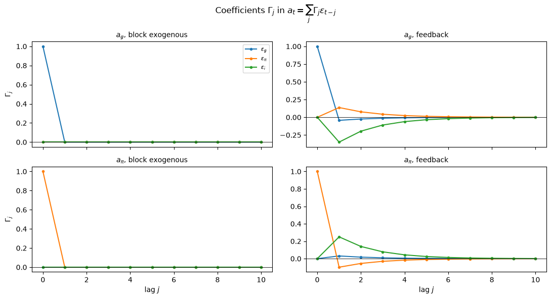
Fig. 48.4 Innovation map coefficients with and without feedback#
In the left column only the \(j = 0\) coefficients are nonzero, and they equal the rows of \(S_y\).
In the right column the omitted interest rate shock \(\varepsilon_i\) leaks into the observed innovations at every lag.
48.9. Summary#
A finite-order VAR for \(Y_t\) implies, for any subvector \(y_t = S_y Y_t\), an infinite-order VAR whose coefficients \(B_j = G(A - KG)^{j-1}K\) come from the steady-state Kalman filter for the companion system.
The innovations of the small system are a one-sided distributed lag \(a_t = \sum_j \Gamma_j \varepsilon_{t-j}\) of the innovations of the large system, with \(\Gamma_j = G(A - KG)^j C\) and \(\Gamma_0 = S_y\).
Because \(\Gamma_j\) is wide, that map cannot be inverted, which is a precise statement of the informational deficiency of a subsystem VAR.
The price is measured by \(\Omega - S_y V S_y^\top = \sum_{j \geq 1} \Gamma_j V \Gamma_j^\top\).
The price is zero when everything is observed, and also when the retained block is block exogenous, in which case the subsystem VAR is exactly the corresponding block of the original one.
48.10. Exercises#
Exercise 48.1
Take the trivariate system of Example 2 and put the feedback of the interest rate onto \((g, \pi)\) under your control by writing
For \(\theta\) on a grid from \(0\) to \(1.5\), plot
\(\det \Omega / \det(S_y V S_y^\top)\), the information lost by dropping \(i_t\),
\(\max_{j \geq 1} |\Gamma_j|\), the size of the leakage of past shocks into the observed innovations.
Explain the shape you find at \(\theta = 0\).
Solution
Here is one solution:
E = np.zeros((3, 3))
E[0, 2], E[1, 2] = -0.35, 0.25

thetas = np.linspace(0, 1.5, 31)
det_ratio, leak = [], []
for th in thetas:
    mod = VARSubsystem([A_exog + th * E], V3, S_gpi)
    Om = mod.innovation_cov()
    det_ratio.append(np.linalg.det(Om)
                     / np.linalg.det(S_gpi @ V3 @ S_gpi.T))
    leak.append(np.abs(mod.innovation_map(40)[1:]).max())

fig, axes = plt.subplots(1, 2, figsize=(11, 4))
axes[0].plot(thetas, det_ratio, lw=2)
axes[0].set(xlabel=r'$\theta$', ylabel='determinant ratio',
            title='information lost by dropping $i_t$')
axes[1].plot(thetas, leak, lw=2, color='C1')
axes[1].set(xlabel=r'$\theta$', ylabel=r'$\max_{j \geq 1} |\Gamma_j|$',
            title='leakage of past shocks into $a_t$')
for ax in axes:
    ax.axhline(ax.get_ylim()[0], color='k', lw=0.6)
fig.tight_layout()
plt.show()

print(f'at theta = 0:   ratio = {det_ratio[0]:.6f}, leakage = {leak[0]:.2e}')
print(f'at theta = 1:   ratio = {det_ratio[20]:.4f}, leakage = {leak[20]:.4f}')
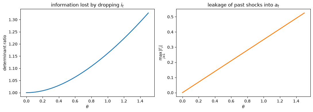
at theta = 0:   ratio = 1.000000, leakage = 1.11e-16
at theta = 1:   ratio = 1.1614, leakage = 0.3500
Both curves start at their minima, exactly zero leakage and a determinant ratio of exactly one.
That is Proposition 48.3: at \(\theta = 0\) the interest rate does not Granger cause \((g, \pi)\), so dropping it costs nothing even though its innovation is contemporaneously correlated with the others.
Both measures rise as the feedback strengthens.
Exercise 48.2
Return to the bivariate system, but replace \(A_1\) and \(A_2\) by the single matrix
so that \(\rho_z\) controls the persistence of the omitted variable \(z\).
Observing \(r\) only, report for \(\rho_z \in \{0.2, 0.5, 0.75, 0.9, 0.95, 0.99\}\)
the forecast error variance \(\Omega\),
the number of lags needed before \(\sum_{j > p} |B_j| < 10^{-3}\).
What does a persistent omitted variable do to the VAR that an econometrician should fit?
Solution
Here is one solution:
print(' rho_z    Omega    lags needed')
for rho_z in [0.2, 0.5, 0.75, 0.9, 0.95, 0.99]:
    mod = VARSubsystem([np.array([[0.5, 0.6], [0.0, rho_z]])],
                       np.eye(2), np.array([[1.0, 0.0]]))
    B = mod.var_coefficients(400)
    tails = [np.abs(B[p:]).sum() for p in range(400)]
    p_need = next(p for p in range(400) if tails[p] < 1e-3)
    print(f' {rho_z:5.2f}   {mod.innovation_cov()[0, 0]:6.4f}      {p_need:3d}')
 rho_z    Omega    lags needed
  0.20   1.3708        3
  0.50   1.4359        5
  0.75   1.5625        5
  0.90   1.6910        7
  0.95   1.7454        8
  0.99   1.7937        8
Both columns rise with \(\rho_z\).
A persistent omitted variable both inflates the forecast error variance and lengthens the autoregression, because the econometrician must reach further back to extract the same information about \(z\) from the history of \(r\).
An empirical VAR with too few lags will therefore be worst exactly where the missing variable is most persistent.
Exercise 48.3
The coefficients \(B_j\) are population objects.
Simulate \(T = 200{,}000\) observations of the bivariate system of Example 1, retain only \(r_t\), and fit finite-order autoregressions of orders \(p = 1, 2, 4, 8\) by ordinary least squares.
Compare the estimates with \(B_1, \ldots, B_p\) and the residual variance with \(\Omega\).
Which order is too short, and what does fitting too short a lag length do to the first coefficient?
Solution
Here is one solution:
Y_big, _ = mod_r.simulate(200_000, seed=3)
r_series = Y_big[:, 0]
B_pop = mod_r.var_coefficients(8)[:, 0, 0]

for p in [1, 2, 4, 8]:
    X = np.column_stack([r_series[p - 1 - l:len(r_series) - 1 - l]
                         for l in range(p)])
    zz = r_series[p:]
    b_hat = np.linalg.lstsq(X, zz, rcond=None)[0]
    resid = zz - X @ b_hat
    print(f'p = {p}')
    print(f'   OLS        {np.round(b_hat, 4)}')
    print(f'   population {np.round(B_pop[:p], 4)}')
    print(f'   residual variance {resid.var():.4f}   Omega {mod_r.innovation_cov()[0, 0]:.4f}')
p = 1
   OLS        [0.8179]
   population [0.7231]
   residual variance 1.6037   Omega 1.5786
p = 2
   OLS        [0.7201 0.1196]
   population [0.7231 0.1212]
   residual variance 1.5807   Omega 1.5786
p = 4
   OLS        [ 0.7207  0.1238 -0.0036 -0.0025]
   population [ 0.7231  0.1212 -0.0056  0.0007]
   residual variance 1.5807   Omega 1.5786
p = 8
   OLS        [ 0.7207  0.1238 -0.0035 -0.0022 -0.0019 -0.0011  0.003   0.0003]
   population [ 0.7231  0.1212 -0.0056  0.0007 -0.0001 -0.     -0.     -0.    ]
   residual variance 1.5806   Omega 1.5786
An AR(1) is too short.
Its single coefficient is pulled well above \(B_1\), because it has to stand in for the omitted second lag, and its residual variance exceeds \(\Omega\).
From \(p = 2\) onward the estimates track the population coefficients and the residual variance settles on \(\Omega\), which matches the finding above that \(B_j\) is negligible beyond the second lag in this example.